Batch Production

Dynamic optimization of bioprocesses: efficient and robust numerical strategies 2003, Julio R. Banga, Eva Balsa-Cantro, Carmen G. Moles and Antonio A. Alonso

Case Study II: Optimal Control of a Fed-Batch Reactor for Ethanol Production

Contents

Problem description

This case study considers a fed-batch reactor for the production of ethanol, as studied by Chen and Hwang (1990a) and others (Bojkov & Luus 1996, Banga et al. 1997). The (free terminal time) optimal control problem is to maximize the yield of ethanol using the feed rate as the control variable. As in the previous case, this problem has been solved using CVP and gradient based methods, but convergence problems have been frequently reported, something which has been confirmed by our own experience. The mathematical statement of the free terminal time problem is:

Find the feed flow rate u(t) and the final time tf over t in [t0; tf ] to maximize

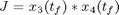
subject to:

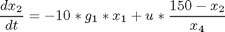
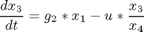
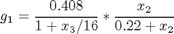
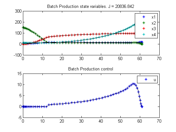
where x1, x2 and x3 are the cell mass, substrate and product concentrations (g/L), and x4 is the volume (L). The initial conditions are:

The constraints (upper and lower bounds) on the control variable (feed rate, L/h) are:

and there is an end-point constraint on the volume:

% Copyright (c) 2007-2008 by Tomlab Optimization Inc.

Problem setup

toms t
toms tfs

tf = 100*tfs;

% initial guesses
tfg = 60;
x1g = 10;
x2g = 150-150*t/tf;
x3g = 70;
x4g = 200*t/tf;
ug  = 3;

n = [  20     60   60   60];
e = [0.01  0.002 1e-4    0];

for i = 1:3

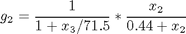
    p = tomPhase('p', t, 0, tf, n(i));
    setPhase(p);

    tomStates x1s x2s x3s x4s
    if e(i)
        tomStates u
    else
        tomControls u
    end
    %tomControls g1 g2

    % Create scaled states, to make the numeric solver work better.
    x1 = 10*x1s;
    x2 = 1*x2s;
    x3 = 100*x3s;
    x4 = 100*x4s;

    % Initial guess
    % Note: The guess for tf must appear in the list before expression involving t.
    x0 = {tf == tfg
        icollocate({
        x1 == x1g
        x2 == x2g
        x3 == x3g
        x4 == x4g
        })
        collocate({u==ug})};

    % Box constraints
    cbox = {
        0.1 <= tf <= 100
        mcollocate({
        0    <= x1
        0    <= x2
        0    <= x3
        1e-8 <= x4  % Avoid division by zero.
        })
        0 <= collocate(u) <= 12};

    % Boundary constraints
    cbnd = {initial({
        x1 == 1;
        x2 == 150
        x3 == 0;
        x4 == 10})
        final(0 <= x4 <= 200)};

    % Various constants and expressions
    g1 = (0.408/(1+x3/16))*(x2/(x2+0.22));
    g2 = (1/(1+x3/71.5))*(x2/(0.44+x2));

    % ODEs and path constraints
    ceq = collocate({
        dot(x1) == g1*x1 - u*x1/x4
        dot(x2) == -10*g1*x1 + u*(150-x2)/x4
        dot(x3) == g2*x1 - u*x3/x4
        dot(x4) == u});

    % Objective
    J = final(x3*x4);
    if e(i)
        % Add cost on oscillating u.
        objective = -J/4900 + e(i)*integrate(dot(u)^2);
    else
        objective = -J/4900;
    end

Solve the problem

    options = struct;
    options.name = 'Batch Production';
    solution = ezsolve(objective, {cbox, cbnd, ceq}, x0, options);

Problem type appears to be: con
===== * * * =================================================================== * * *
TOMLAB - Tomlab Optimization Inc. Development license  999001. Valid to 2010-02-05
=====================================================================================
Problem: ---  1: Batch Production               f_k      -4.151115744681614000
                                       sum(|constr|)      0.259618778556077960
                              f(x_k) + sum(|constr|)     -3.891496966125536100
                                              f(x_0)      1.259999999999963600

Solver: snopt.  EXIT=1.  INFORM=32.
SNOPT 7.2-5 NLP code
Major iteration limit reached

FuncEv 4890 GradEv 4888 ConstrEv 4888 ConJacEv 4888 Iter 1000 MinorIter 4377
CPU time: 21.343750 sec. Elapsed time: 21.703000 sec. 

Problem type appears to be: con
===== * * * =================================================================== * * *
TOMLAB - Tomlab Optimization Inc. Development license  999001. Valid to 2010-02-05
=====================================================================================
Problem: ---  1: Batch Production               f_k      -4.222925110913788400
                                       sum(|constr|)      0.000001041586989401
                              f(x_k) + sum(|constr|)     -4.222924069326799300
                                              f(x_0)     -1.852183384354953300

Solver: snopt.  EXIT=0.  INFORM=1.
SNOPT 7.2-5 NLP code
Optimality conditions satisfied

FuncEv  597 GradEv  595 ConstrEv  595 ConJacEv  595 Iter  547 MinorIter 1080
CPU time: 20.078125 sec. Elapsed time: 20.484000 sec. 

Problem type appears to be: con
===== * * * =================================================================== * * *
TOMLAB - Tomlab Optimization Inc. Development license  999001. Valid to 2010-02-05
=====================================================================================
Problem: ---  1: Batch Production               f_k      -4.248461991804581400
                                       sum(|constr|)      0.000004064043825988
                              f(x_k) + sum(|constr|)     -4.248457927760755500
                                              f(x_0)     -4.126187506167310600

Solver: snopt.  EXIT=0.  INFORM=1.
SNOPT 7.2-5 NLP code
Optimality conditions satisfied

FuncEv  333 GradEv  331 ConstrEv  331 ConJacEv  331 Iter  159 MinorIter  629
CPU time: 6.921875 sec. Elapsed time: 7.062000 sec. 

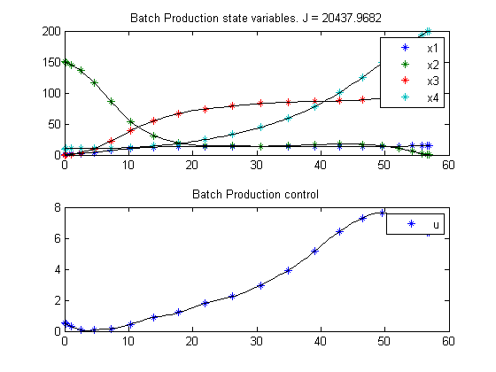
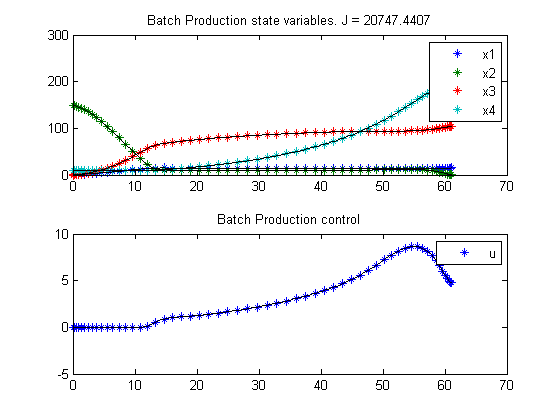
Plot result

    subplot(2,1,1)
    ezplot([x1 x2 x3 x4]);
    legend('x1','x2','x3','x4');
    title(['Batch Production state variables. J = ' num2str(subs(J,solution))]);

    subplot(2,1,2)
    ezplot(u);
    legend('u');
    title('Batch Production control');
    drawnow

    % Copy inital guess for next iteration
    tfg = subs(tf,solution);
    x1g = subs(x1,solution);
    x2g = subs(x2,solution);
    x3g = subs(x3,solution);
    x4g = subs(x4,solution);

end