The Brachistochrone Problem (DAE formulation)
We will now solve the same problem as in brachistochrone.m, but using a DAE formulation for the mechanics.
Contents
DAE formulation
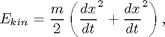
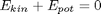
In a DAE formulation we don't need to formulate explicit equations for the time-derivatives of each state. Instead we can, for example, formulate the conservation of energy.

The boundary conditions are still A = (0,0), B = (10,-3), and an initial speed of zero, so we have
For complex mechanical systems, this freedom to choose the most convenient formulation can save a lot of effort in modelling the system. On the other hand, computation times may get longer, because the problem can to become more non-linear and the jacobian less sparse.
% Copyright (c) 2007-2008 by Tomlab Optimization Inc.
Problem setup
toms t
toms tf

p = tomPhase('p', t, 0, tf, 20);
setPhase(p);

tomStates x y

% Initial guess
x0 = {tf == 10};

% Box constraints
cbox = {0.1 <= tf <= 100};

% Boundary constraints
cbnd = {initial({x == 0; y == 0})
    final({x == 10; y == -3})};

% Expressions for kinetic and potential energy
m = 1;
g = 9.81;
Ekin = 0.5*m*(dot(x).^2+dot(y).^2);
Epot = m*g*y;
v = sqrt(2/m*Ekin);

% ODEs and path constraints
ceq = collocate(Ekin + Epot == 0);

% Objective
objective = tf;
Solve the problem
options = struct;
options.name = 'Brachistochrone-DAE';
solution = ezsolve(objective, {cbox, cbnd, ceq}, x0, options);
x  = subs(collocate(x),solution);
y  = subs(collocate(y),solution);
v  = subs(collocate(v),solution);
t  = subs(collocate(t),solution);
Problem type appears to be: lpcon
===== * * * =================================================================== * * *
TOMLAB - Tomlab Optimization Inc. Development license  999001. Valid to 2010-02-05
=====================================================================================
Problem: ---  1: Brachistochrone-DAE            f_k       1.869963310228403700
                                       sum(|constr|)      0.000000000838561570
                              f(x_k) + sum(|constr|)      1.869963311066965300
                                              f(x_0)     10.000000000000000000

Solver: snopt.  EXIT=0.  INFORM=1.
SNOPT 7.2-5 NLP code
Optimality conditions satisfied

FuncEv    1 ConstrEv  169 ConJacEv  169 Iter   99 MinorIter  160
CPU time: 0.218750 sec. Elapsed time: 0.219000 sec.
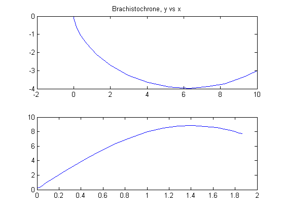
Plot the result
To obtain the brachistochrone curve, we plot y versus x.
subplot(2,1,1)
plot(x, y);
title('Brachistochrone, y vs x');

subplot(2,1,2)
plot(t, v);