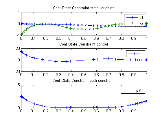
Continuous State Constraint Problem
Problem 2: Miser3 manual
Contents
Problem description
Find u(t) over t in [0; 1 ] to minimize

subject to:


% Copyright (c) 2007-2008 by Tomlab Optimization Inc.
Problem setup
toms t
p = tomPhase('p', t, 0, 1, 50);
setPhase(p);

tomStates x1 x2
tomControls u

% Initial guess
x0 = {icollocate({x1 == 0; x2 == -1})
    collocate(u==0)};

% Box constraints
cbox = {-10 <= icollocate(x1) <= 10
    -10 <= icollocate(x2) <= 10
    -20 <= collocate(u)  <= 20};

% Boundary constraints
cbnd = initial({x1 == 0; x2 == -1});

% ODEs and path constraints
ceq = collocate({
    dot(x1) == x2
    dot(x2) == -x2+u
    8*(t-0.5).^2-0.5-x2 >= 0 % Path constr.
    });

% Objective
objective = integrate(x1.^2 + x2.^2 + 0.005*u.^2);
Solve the problem
options = struct;
options.name = 'Cont State Constraint';
solution = ezsolve(objective, {cbox, cbnd, ceq}, x0, options);
t  = subs(collocate(t),solution);
x1 = subs(collocate(x1),solution);
x2 = subs(collocate(x2),solution);
u  = subs(collocate(u),solution);
Problem type appears to be: qp
===== * * * =================================================================== * * *
TOMLAB - Tomlab Optimization Inc. Development license  999001. Valid to 2010-02-05
=====================================================================================
Problem:  1: Cont State Constraint              f_k       0.169824305998486440
                                       sum(|constr|)      0.000000000079816838
                              f(x_k) + sum(|constr|)      0.169824306078303290
                                              f(x_0)      0.000000000000000000

Solver: CPLEX.  EXIT=0.  INFORM=1.
CPLEX Barrier QP solver
Optimal solution found

FuncEv   10 GradEv   10 ConstrEv   10 Iter   10
CPU time: 0.015625 sec. Elapsed time: 0.015000 sec.
Plot result
subplot(3,1,1)
plot(t,x1,'*-',t,x2,'*-');
legend('x1','x2');
title('Cont State Constraint state variables');

subplot(3,1,2)
plot(t,u,'+-');
legend('u');
title('Cont State Constraint control');

subplot(3,1,3)
ieq = 8*(t-0.5).^2-0.5-x2;
plot(t,ieq,'+-');
axis([0 1 0 5]);
legend('path');
title('Cont State Constraint path constraint');
