Lee-Ramirez Bioreactor
Dynamic optimization of chemical and biochemical processes using restricted second-order information 2001, Eva Balsa-Canto, Julio R. Banga, Antonio A. Alonso Vassilios S. Vassiliadis
Case Study II: Lee-Ramirez bioreactor
Contents
Problem description
This problem considers the optimal control of a fed-batch reactor for induced foreign protein production by recombinant bacteria, as presented by Lee and Ramirez (1994) and considered afterwards by Tholudur and Ramirez (1997) and Carrasco and Banga (1998). The objective is to maximize the profitability of the process using the nutrient and the inducer feeding rates as the control variables. Three different values for the ratio of the cost of inducer to the value of the protein production (Q) were considered.
The mathematical formulation, following the modified parameter function set presented by Tholudur and Ramirez (1997) to increase the sensitivity to the controls, is as follows:
Find u1(t) and u2(t) over t in [t0 tf] to maximize:
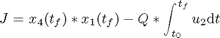
subject to:

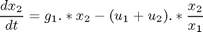
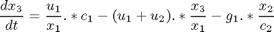
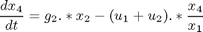
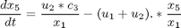
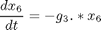
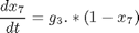
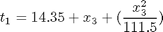

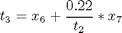
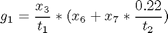


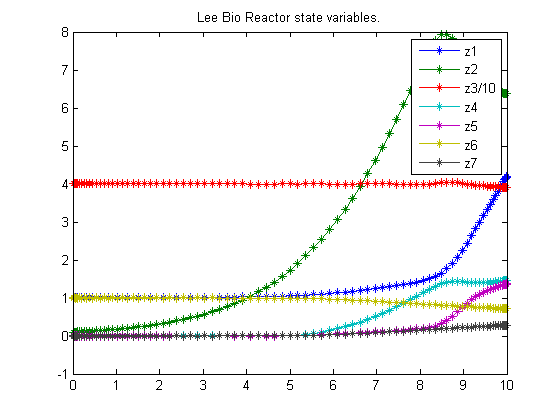
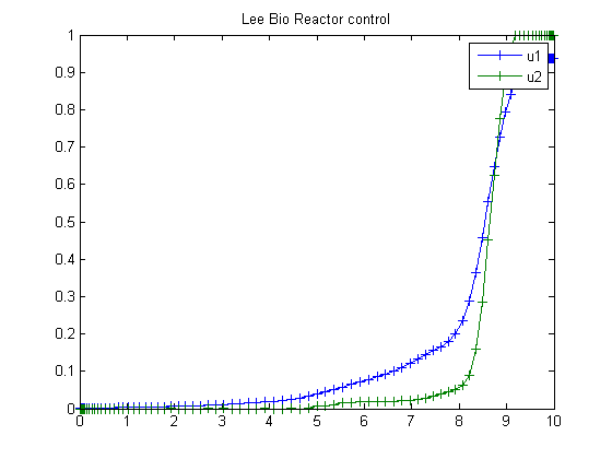
where the state variables are the reactor volume (x1), the cell density (x2), the nutrient concentration (x3), the foreign protein concentration (x4), the inducer concentration (x5), the inducer shock factor on cell growth rate (x6) and the inducer recovery factor on cell growth rate (x7). The two control variables are the glucose rate (u1) and the inducer feeding rate (u2). Q is the ratio of the cost of inducer to the value of the protein production, and the final time is considered fixed as tf = 10 h. The model parameters were described by Lee and Ramirez (1994). The initial conditions are:
![$$ x(t_0) = [1 \ 0.1 \ 40 \ 0 \ 0 \ 1 \ 0]' $$](xleeBioReactor_eq98997.png)
The following constraints on the control variables are considered:


% Copyright (c) 2007-2008 by Tomlab Optimization Inc.
Problem setup
toms t

for n=[20 35 55 85]
    p = tomPhase('p', t, 0, 10, n);
    setPhase(p);

    tomStates z1 z2 z3s z4 z5 z6 z7

    % Declaring u as "states" makes it possible to work with their
    % derivatives.
    tomStates u1 u2

    % Scale z3 by 40
    z3 = z3s*40;

    % Initial guess
    if n == 20
        x0 = {icollocate({z1 == 1; z2 == 0.1
            z3 == 40; z4 == 0; z5 == 0
            z6 == 1; z7 == 0})
            icollocate({u1==t/10; u2==t/10})};
    else
        x0 = {icollocate({z1 == z1opt
            z2 == z2opt; z3 == z3opt
            z4 == z4opt; z5 == z5opt
            z6 == z6opt; z7 == z7opt})
            icollocate({u1 == u1opt
            u2 == u2opt})};
    end

    % Box constraints
    cbox = {mcollocate({0 <= z1; 0 <= z2
        0 <= z3; 0 <= z4; 0 <= z5})
        0 <= collocate(u1) <= 1
        0 <= collocate(u2) <= 1};

    % Boundary constraints
    cbnd = initial({z1 == 1; z2 == 0.1
        z3 == 40; z4 == 0; z5 == 0
        z6 == 1; z7 == 0});

    % Various constants and expressions
    c1 = 100; c2 = 0.51; c3 = 4.0;
    Q  = 0;

    t1 = 14.35+z3+((z3).^2/111.5);
    t2 = 0.22+z5;
    t3 = z6+0.22./t2.*z7;

    g1 = z3./t1.*(z6+z7*0.22./t2);
    g2 = 0.233*z3./t1.*((0.0005+z5)./(0.022+z5));
    g3 = 0.09*z5./(0.034+z5);

    % ODEs and path constraints
    ceq = collocate({
        dot(z1) == u1+u2
        dot(z2) == g1.*z2-(u1+u2).*z2./z1
        dot(z3) == u1./z1.*c1-(u1+u2).*z3./z1-g1.*z2/c2
        dot(z4) == g2.*z2-(u1+u2).*z4./z1
        dot(z5) == u2*c3./z1-(u1+u2).*z5./z1
        dot(z6) == -g3.*z6
        dot(z7) == g3.*(1-z7)});

    % Objective
    J = -final(z1)*final(z4)+Q*integrate(u2);

    damp = 0.1/n; % penalty term to yield a smoother u.
    objective = J + damp*integrate(dot(u1)^2+dot(u2)^2);
Solve the problem
    options = struct;
    options.name = 'Lee Bio Reactor';
    solution = ezsolve(objective, {cbox, cbnd, ceq}, x0, options);

    % Optimal z, u for starting point
    z1opt = subs(z1, solution);
    z2opt = subs(z2, solution);
    z3opt = subs(z3, solution);
    z4opt = subs(z4, solution);
    z5opt = subs(z5, solution);
    z6opt = subs(z6, solution);
    z7opt = subs(z7, solution);
    u1opt = subs(u1, solution);
    u2opt = subs(u2, solution);
Problem type appears to be: qpcon
===== * * * =================================================================== * * *
TOMLAB - Tomlab Optimization Inc. Development license  999001. Valid to 2010-02-05
=====================================================================================
Problem: ---  1: Lee Bio Reactor                f_k      -6.158549893842515400
                                       sum(|constr|)      0.000001696596070549
                              f(x_k) + sum(|constr|)     -6.158548197246444600
                                              f(x_0)      0.000999999999999945

Solver: snopt.  EXIT=0.  INFORM=1.
SNOPT 7.2-5 NLP code
Optimality conditions satisfied

FuncEv    1 ConstrEv  688 ConJacEv  688 Iter  529 MinorIter 3450
CPU time: 6.609375 sec. Elapsed time: 6.750000 sec.
Problem type appears to be: qpcon
===== * * * =================================================================== * * *
TOMLAB - Tomlab Optimization Inc. Development license  999001. Valid to 2010-02-05
=====================================================================================
Problem: ---  1: Lee Bio Reactor                f_k      -6.149281026758400200
                                       sum(|constr|)      0.000000113027662584
                              f(x_k) + sum(|constr|)     -6.149280913730737400
                                              f(x_0)     -6.161231516476529900

Solver: snopt.  EXIT=0.  INFORM=1.
SNOPT 7.2-5 NLP code
Optimality conditions satisfied

FuncEv    1 ConstrEv  512 ConJacEv  512 Iter  462 MinorIter 1514
CPU time: 12.765625 sec. Elapsed time: 13.031000 sec.
Problem type appears to be: qpcon
===== * * * =================================================================== * * *
TOMLAB - Tomlab Optimization Inc. Development license  999001. Valid to 2010-02-05
=====================================================================================
Problem: ---  1: Lee Bio Reactor                f_k      -6.148471246836187700
                                       sum(|constr|)      0.000003449359665746
                              f(x_k) + sum(|constr|)     -6.148467797476522300
                                              f(x_0)     -6.151340399353863100

Solver: snopt.  EXIT=0.  INFORM=1.
SNOPT 7.2-5 NLP code
Optimality conditions satisfied

FuncEv    1 ConstrEv  263 ConJacEv  263 Iter  232 MinorIter 1318
CPU time: 20.609375 sec. Elapsed time: 20.906000 sec.
Problem type appears to be: qpcon
===== * * * =================================================================== * * *
TOMLAB - Tomlab Optimization Inc. Development license  999001. Valid to 2010-02-05
=====================================================================================
Problem: ---  1: Lee Bio Reactor                f_k      -6.149330995342836600
                                       sum(|constr|)      0.000001492539524976
                              f(x_k) + sum(|constr|)     -6.149329502803311700
                                              f(x_0)     -6.149416170638048100

Solver: snopt.  EXIT=0.  INFORM=1.
SNOPT 7.2-5 NLP code
Optimality conditions satisfied

FuncEv    1 ConstrEv  912 ConJacEv  912 Iter  818 MinorIter 3515
CPU time: 299.031250 sec. Elapsed time: 304.265000 sec.
end

t  = subs(collocate(t),solution);
z1 = subs(collocate(z1),solution);
z2 = subs(collocate(z2),solution);
z3 = subs(collocate(z3),solution);
z4 = subs(collocate(z4),solution);
z5 = subs(collocate(z5),solution);
z6 = subs(collocate(z6),solution);
z7 = subs(collocate(z7),solution);
u1 = subs(collocate(u1),solution);
u2 = subs(collocate(u2),solution);
Plot result
figure(1)
plot(t,z1,'*-',t,z2,'*-',t,z3/10,'*-',t,z4,'*-' ...
    ,t,z5,'*-',t,z6,'*-',t,z7,'*-');
legend('z1','z2','z3/10','z4','z5','z6','z7');
title('Lee Bio Reactor state variables.');

figure(2)
plot(t,u1,'+-',t,u2,'+-');
legend('u1','u2');
title('Lee Bio Reactor control');

disp('J = ');
disp(subs(J,solution));
J =
   -6.1510