Tubular Reactor
Global Optimization of Chemical Processes using Stochastic Algorithms 1996, Julio R. Banga, Warren D. Seider
Case Study V: Global optimization of a bifunctional catalyst blend in a tubular reactor
Contents
Problem Description
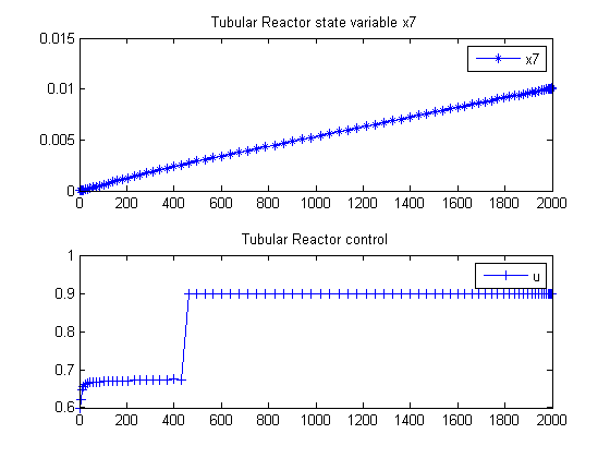
Luus et al and Luus and Bojkov consider the optimization of a tubular reactor in which methylcyclopentane is converted into benzene. The blend of two catalysts, for hydrogenation and isomerization is described by the mass fraction u of the hydrogenation catalyst. The optimal control problem is to find the catalyst blend along the length of the reactor defined using a characteristic reaction time t in the interval 0 <= t <= tf where tf = 2000 gh/mol corresponding to the reactor exit such that the benzene concentration at the exit of the reactor is maximized.
Find u(t) to maximize:

Subject to:


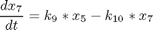
where xi, i = 1,..,7 are the mole fractions of the chemical species (i = 1 for methylcyclopentane, i = 7 for benzene), the rate constants are functions of the catalyst blend u(t):

and the coefficients cij are given by Luus et al. The upper and lower bounds on the mass fraction of the hydrogenation catalyst are.

The initial vector of mole fractions is:
![$$ x(t_0) = [1 \ 0 \ 0 \ 0 \ 0 \ 0 \ 0]' $$](xtubularReactor_eq67765.png)
% Copyright (c) 2007-2008 by Tomlab Optimization Inc.

% Data
c = [0.2918487e-2, -0.8045787e-2, 0.6749947e-2,  -0.1416647e-2;...
    0.9509977e1,   -0.3500994e2,  0.4283329e2,   -0.1733333e2; ...
    0.2682093e2,   -0.9556079e2,  0.1130398e3,   -0.4429997e2; ...
    0.2087241e3,   -0.7198052e3,  0.8277466e3,   -0.3166655e3; ...
    0.1350005e1,   -0.6850027e1,  0.1216671e2,   -0.6666689e1; ...
    0.1921995e-1,  -0.7945320e-1, 0.1105666,     -0.5033333e-1;...
    0.1323596,     -0.4696255,    0.5539323,     -0.2166664;   ...
    0.7339981e1,   -0.2527328e2,  0.2993329e2,   -0.1199999e2; ...
    -0.3950534,     0.1679353e1,  -0.1777829e1,  0.4974987;    ...
    -0.2504665e-4,  0.1005854e-1, -0.1986696e-1, 0.9833470e-2]';

% Independent variable
toms t

% Initial guess
x1opt = 1; x2opt = 0;
x3opt = 0; x4opt = 0;
x5opt = 0; x6opt = 0;
x7opt = 0; uopt = 0.9;

% Loop over number of collocation points
for n=[10 80]
Problem setup
    p = tomPhase('p', t, 0, 2000, n);
    setPhase(p);

    tomStates x1 x2 x3 x4 x5 x6 x7
    tomControls u

    % Collocate initial guess
    x0 = {icollocate({x1 == x1opt; x2 == x2opt
        x3 == x3opt; x4 == x4opt; x5 == x5opt
        x6 == x6opt; x7 == x7opt})
        collocate(u == uopt)};

    % Box constraints
    cbox = {icollocate({
        0 <= x1 <= 1; 0 <= x2 <= 1
        0 <= x3 <= 1; 0 <= x4 <= 1
        0 <= x5 <= 1; 0 <= x6 <= 1
        0 <= x7 <= 1})
        0.6 <= collocate(u) <= 0.9};

    % Boundary constraints
    cbnd = initial({x1 == 1; x2 == 0
        x3 == 0; x4 == 0; x5 == 0
        x6 == 0; x7 == 0});

    % ODEs and path constraints
    uvec = [1, u, u.^2, u.^3];
    k    = (c'*uvec')';
    ceq = collocate({
        dot(x1) == -k(1)*x1
        dot(x2) ==  k(1)*x1-(k(2)+k(3))*x2+k(4)*x5
        dot(x3) ==  k(2)*x2
        dot(x4) == -k(6)*x4+k(5)*x5
        dot(x5) ==  k(3)*x2+k(6)*x4-(k(4)+k(5)+k(8)+k(9))*x5+...
        k(7)*x6+k(10).*x7
        dot(x6) == k(8)*x5-k(7)*x6
        dot(x7) == k(9)*x5-k(10)*x7});

    % Objective
    objective = -final(x7);
    options = struct;
    options.name = 'Tubular Reactor';
    options.d2c = false;
    Prob = sym2prob('con',objective,{cbox, cbnd, ceq}, x0, options);
    Prob.xInit = 35; % Use 35 random starting points.
    Prob.GO.localSolver = 'snopt';
    if n<=10
        Result = tomRun('multiMin', Prob, 1);
    else
        Result = tomRun('snopt', Prob, 1);
    end
    solution = getSolution(Result);

    % Store optimum for use in initial guess
    x1opt = subs(x1,solution);
    x2opt = subs(x2,solution);
    x3opt = subs(x3,solution);
    x4opt = subs(x4,solution);
    x5opt = subs(x5,solution);
    x6opt = subs(x6,solution);
    x7opt = subs(x7,solution);
    uopt  = subs(u,solution);
===== * * * =================================================================== * * *
TOMLAB - Tomlab Optimization Inc. Development license  999001. Valid to 2010-02-05
=====================================================================================
Problem: ---  1: Tubular Reactor                f_k      -0.010093482963145356
                                       sum(|constr|)      0.000000004467202512
                              f(x_k) + sum(|constr|)     -0.010093478495942844
                                              f(x_0)     -1.010438967758588500

Solver: multiMin with local solver snopt.  EXIT=0.  INFORM=1.
Find local optima using multistart local search
Did 35 local tries. Found 31 local minima

FuncEv   31 GradEv   29 ConstrEv   29 ConJacEv   29 Iter   19 MinorIter  204
CPU time: 5.312500 sec. Elapsed time: 5.359000 sec.
===== * * * =================================================================== * * *
TOMLAB - Tomlab Optimization Inc. Development license  999001. Valid to 2010-02-05
=====================================================================================
Problem: ---  1: Tubular Reactor                f_k      -0.010082374590765433
                                       sum(|constr|)      0.000000000045366255
                              f(x_k) + sum(|constr|)     -0.010082374545399177
                                              f(x_0)     -0.010093482963145358

Solver: snopt.  EXIT=0.  INFORM=1.
SNOPT 7.2-5 NLP code
Optimality conditions satisfied

FuncEv   51 GradEv   49 ConstrEv   49 ConJacEv   49 Iter   34 MinorIter  490
CPU time: 4.953125 sec. Elapsed time: 5.062000 sec.
end
Plot result
t  = collocate(t);
x7 = collocate(x7opt);
u  = collocate(uopt);

subplot(2,1,1)
plot(t,x7,'*-');
legend('x7');
title('Tubular Reactor state variable x7');

subplot(2,1,2)
plot(t,u,'+-');
legend('u');
title('Tubular Reactor control');